By Kevin Collins and Alejandro Frydman
This year, like in past years, we conducted several internally-funded state-level polls as part of our ongoing methodology R&D program. This year, for the first time, we put out public estimates in advance of Election Day a week ago. (In addition to our website, you can also find these estimates aggregated by external news sites). This year we surveyed Kansas, Minnesota, Ohio, and Maine, to create a relatively geographically diverse (but plausibly competitive) set of states with contests for both Governor and United States Senate.
Overall, our surveys were accurate in a year where poll averages substantially underestimated Democratic performance. Averaging across senate and governor races in the four states, our likely voter estimates underestimated Democratic vote share by 1.4 percentage points on average.
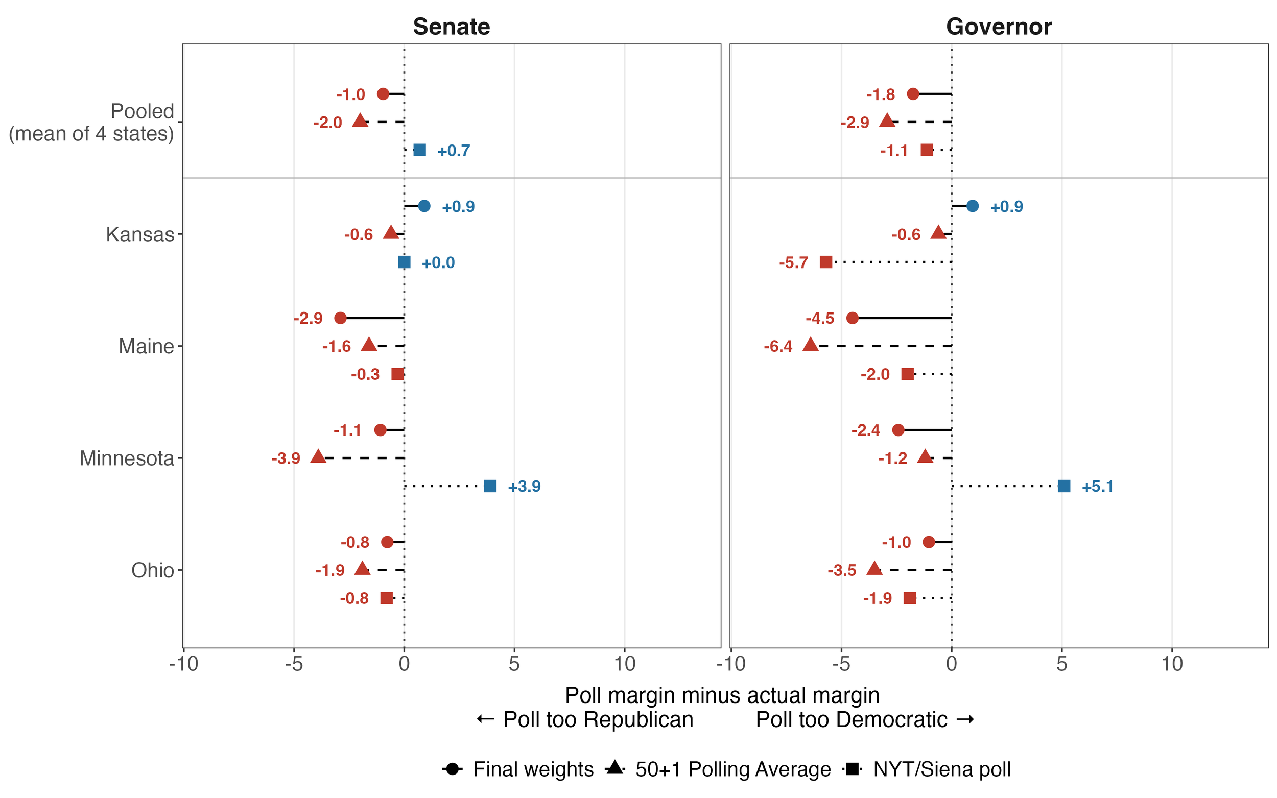
As the graph below shows, our estimates were closer to the election results than the FiftyPlusOne poll averages in five of the eight contests. Compared to the final New York Times/Siena polls in the same states, we were more accurate in four contests, equally accurate in one, and less accurate in three. Across all eight races, the mean absolute error was 1.8 percentage points in our surveys, 2.5 pp for the FiftyPlusOne poll averages, and 2.5 pp for the New York Times/Siena polls. Pollster performance assessments will surely be coming out in the coming weeks, but we are confident that our performance will stand out.
Yet the purpose of this review is not to see how we compare to others, but is instead to evaluate the methodological decisions we made and to identify ways to keep improving. To do that, we must first briefly describe those methodological choices.
Our Methodology
This year, in addition to our texting tools to reach voters who had a cell phone number available, we used automated calling tools to reach records with only landline phone numbers available on the L2 voter file (which we used for sampling). We drew a stratified sample from that file (which were defined by race, age, participation in the 2024 general election, L2’s party alignment, and L2’s educational attainment categorical model) with proportions adjusted to account for expected response rates. We also used our Dynamic Response-rate Adjusted Stratified Sampling (DRASS) algorithm built into our text message survey platform to help keep the distribution of responses across strata aligned with the population distribution of those strata.
We then weighted the data (using raking, also known as iterative and proportional fitting) to our registered voter sample, and likely voters were identified from within that weighted sample. Weighting factors included:
- The distribution of sampling strata.
- Self-reported educational attainment, weighted to estimates from the 2024 Current Population Survey (CPS) November Supplement’s estimates for registered voters in each state
- Early vote, using self-reported early voting and weighting the share of registered voters in each state who had voted early, as reported by each state’s Secretary of State’s office.
- Self-reported 2024 vote, using as weighting targets the share of 2024 non-voters among current voter registration list and then multiplying through the 2024 vote share through the proportion of people who did vote in 2024. We also re-code anyone as a non-voter who reported voting for a candidate but does not show up as a 2024 voter on the voter file.
- Mode of interview, weighting to the proportion of records with only a landline in the L2 file of those with any phone number available at all.
Reviewing these decisions by comparing our final (and also, counterfactual) estimates against actual results, we have several takeaways.
Takeaway #1: Reaching landlines in addition to cellphones improved survey performance on average.
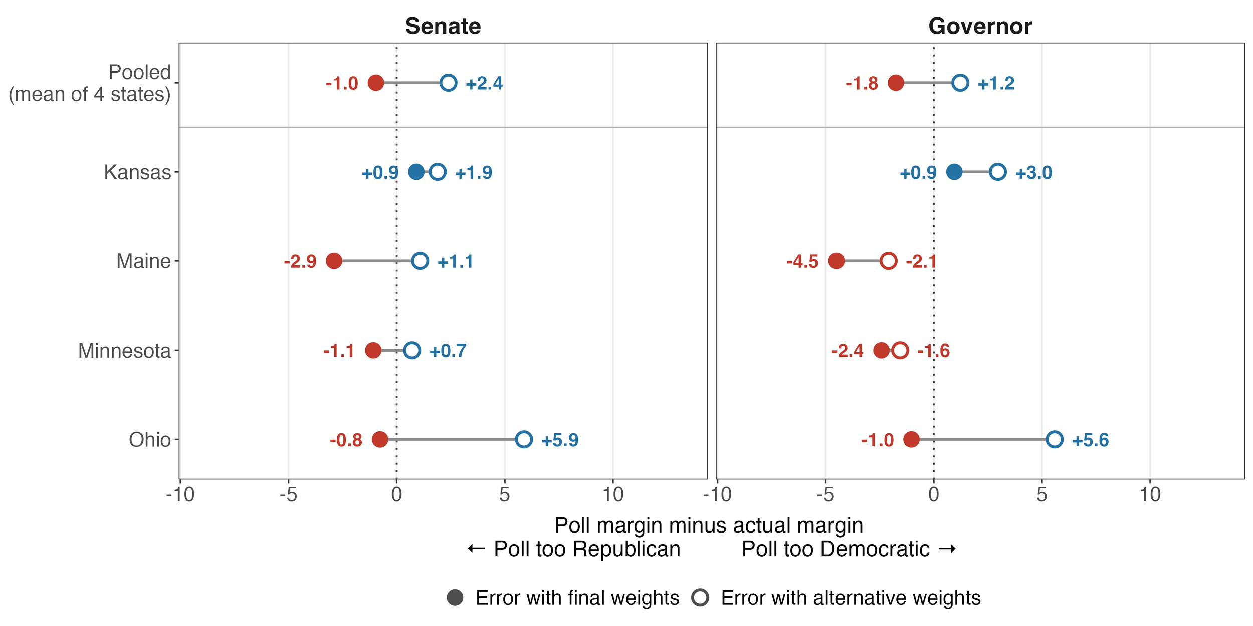
While we focus on text message surveys, we are proponents of multimodal approaches to reduce coverage error. This is why we used automated calling tools to reach landlines for these surveys. Unfortunately, the response rates for these automated calls to landlines were quite low —even lower than anticipated — which necessitated weighting up landlines (and increasing the design effect as a result). The graph below illustrates this by showing our final estimates compared to a final estimate that excluded landlines and did not weight to them. We see that this counterfactual without landlines was more accurate in Maine and (slightly) Minnesota, but on average the results would have been worse without the multi-modal approach.
In the future, we anticipate either using other ways to reach landlines to improve response rates and/or oversampling landlines to account for these low response rates to avoid needing to weight up this portion of the sample so dramatically.
Takeaway #2: Weighting by recalled 2024 vote choice improved accuracy on average.
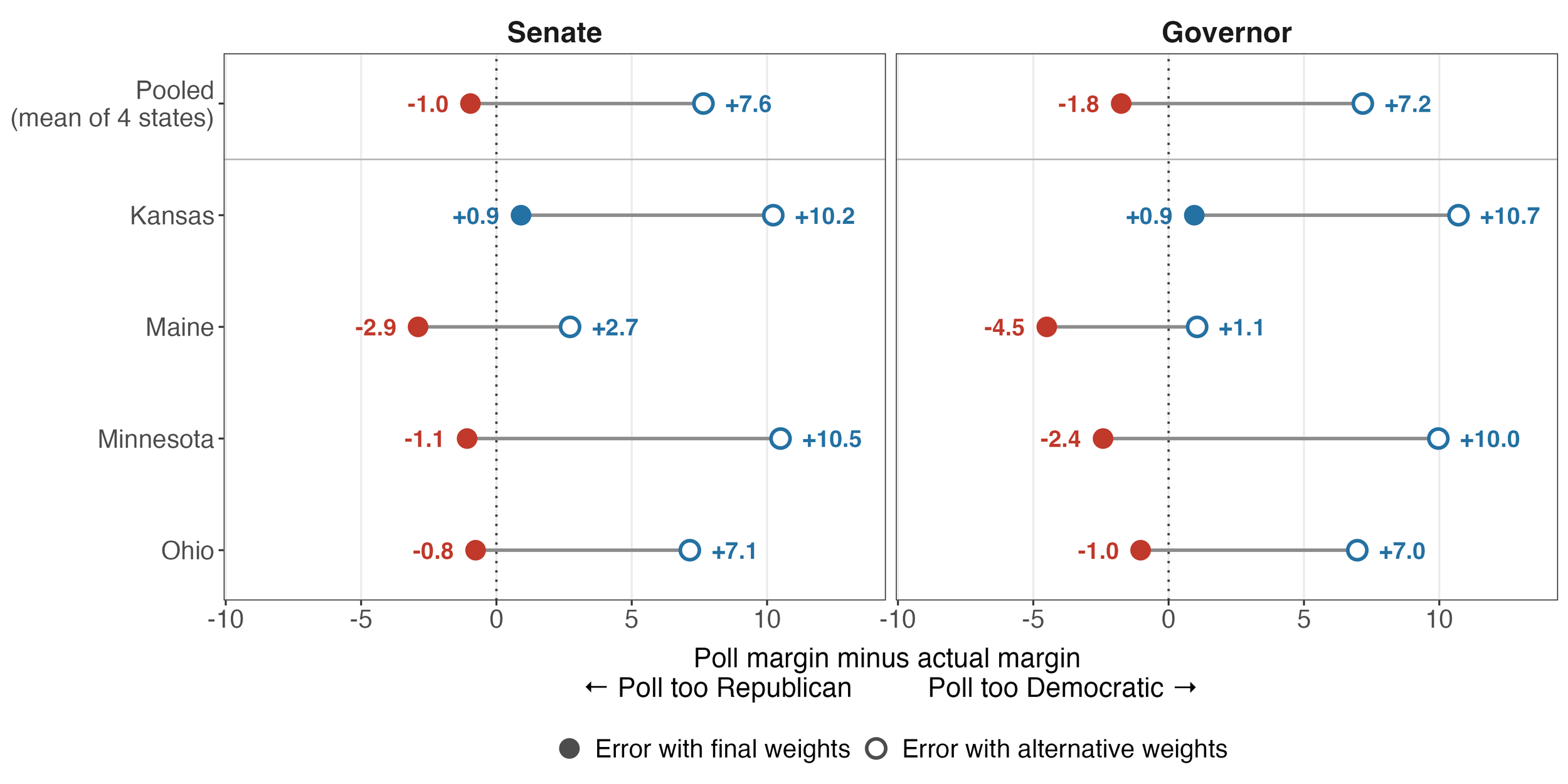
One of the more controversial topics within the survey research industry is whether to weight on recalled past vote choice in the previous presidential election. The New York Times/Siena polls didn’t do this for a long time (until they did). And as G. Elliott Morris has pointed out, a small but meaningful proportion of respondents in panels misreport their past vote, compared to contemporaneous measures of that 2024 vote choice. However, we find including the weight (as defined above) increased accuracy dramatically in three of the four states polled as well as on average, as shown in the graphs below.
Going forward, we intend to build on this success by exploring weighting on recalled vote in multiple previous elections (such as the one we just had), and building better weighting targets to account for shifts in the electorate. While the approach we adopted in this cycle explicitly allowed for more new registrants (who could not have voted in 2026), we are exploring strategies for adjusting the weighting targets to account for inter-state movers or past voters aging out of the current electorate.
Takeaway #3: Including early vote weights slightly reduced accuracy on average.
As a general practice, there are at least three criteria for what makes for a good weighting variable: correlated with non-response, correlated with outcomes of interest, and well-measured. When fielding the survey, we observed that respondents were reporting having already voted at higher rates than the rates at which states were reporting early vote as a share of registered voters, suggesting that early voting is correlated with response rate. We also saw that these voters had a partisan lean. And so we thought it was a good idea to add this as a voting weight.
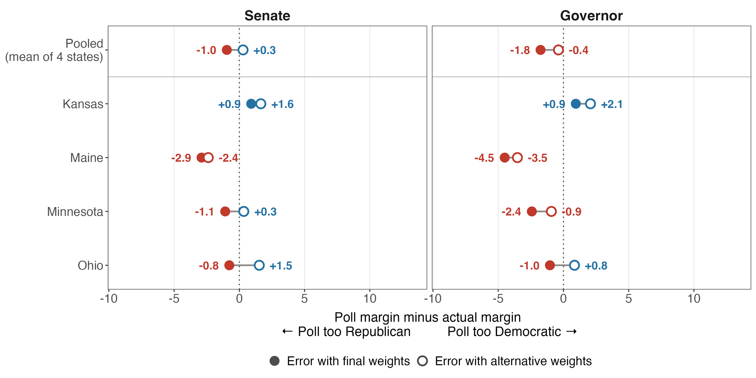
In the graph below, we show the final weights with early vote weights to counterfactual estimates without the early vote weights. While the final weights with early voting weights were more accurate in Kansas, in the other three states (and on average) the counterfactual weights were slightly more accurate. Overall, if we had skipped weighting by early vote, that would have brought our bias to close to 0 (-0.049) across the eight races, and reduced our mean absolute error from 1.8 to 1.7 percentage points.
Based on this analysis, our approach going forward will not include early vote weights. Among other reasons, we believe that this variable was not measured with sufficient accuracy or reliability. The reference value for the weight – the proportion of registered voters in the state that voted early – literally changes over the course of the survey as more people vote early. And two of these states (Maine and Minnesota) had same day registration, meaning the denominator changes as well. Perhaps coincidentally, those are the two states where excluding early vote weights would have improved accuracy in both contests. Additionally, people who said they hadn’t voted already may have cast an early ballot before the survey was out of the field. And that is before accounting for the fact that some people who tell us that they have already voted in fact did not.
An alternative way to weight on early voting would be to use official state records of early voting, but those can take multiple days to update, especially for mail ballots, which would delay the release (and make it impossible to field a survey immediately before the election, as we did here). Instead, we will explore early voting in previous elections as a weighting variable (and in the future, this will be one of those previous elections), where the voter file provides both the individual measure and the weighting target, avoiding the measurement problems discussed here.
Appendix: Detailed Poll Estimates
For maximum transparency, the table below reports the estimates and election results that were used in the calculation of our polling error. In this table we report our likely vote estimate to the first decimal places. While we generally do not report polling estimates to the decimal place, because that overstates the precision of the estimates, we believe this is useful for calculating polling error against vote shares that can be reported at that level of precision to avoid conflating rounding with error.
| Survey 160 Polls (LV) | Result | Margin error | ||||||
|---|---|---|---|---|---|---|---|---|
| D | R | Margin | D | R | Margin | Signed | Absolute | |
| Senate | ||||||||
| Kansas | 50.0 | 44.1 | +5.9 | 51.0 | 46.0 | +5.0 | +0.9 | 0.9 |
| Maine | 50.1 | 46.7 | +3.4 | 53.1 | 46.8 | +6.3 | -2.9 | 2.9 |
| Minnesota | 52.4 | 43.4 | +9.0 | 53.7 | 43.6 | +10.1 | -1.1 | 1.1 |
| Ohio | 49.6 | 45.6 | +4.0 | 50.0 | 45.2 | +4.8 | -0.8 | 0.8 |
| Governor | ||||||||
| Kansas | 49.5 | 47.8 | +1.6 | 50.4 | 49.7 | +0.7 | +0.9 | 0.9 |
| Maine | 53.3 | 40.8 | +12.5 | 54.4 | 37.4 | +17.0 | -4.5 | 4.5 |
| Minnesota | 53.4 | 42.9 | +10.5 | 55.5 | 42.6 | +12.9 | -2.4 | 2.4 |
| Ohio | 50.8 | 44.0 | +6.9 | 52.3 | 44.4 | +7.9 | -1.0 | 1.0 |
| Average (8 races) | -1.4 | 1.8 | ||||||
Note: Election results current as of 11/9 at 1:00 PM EST.